Excel Made Easy

Add small table to a cell with sparkline in Excel

For example, it is very difficult for Management to review the performance from raw data table as it is. Is there a way to make the data more easily interpretable?

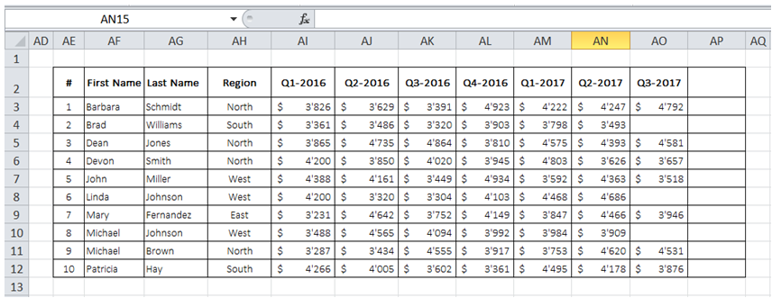
To do it in Excel, here is the answer:

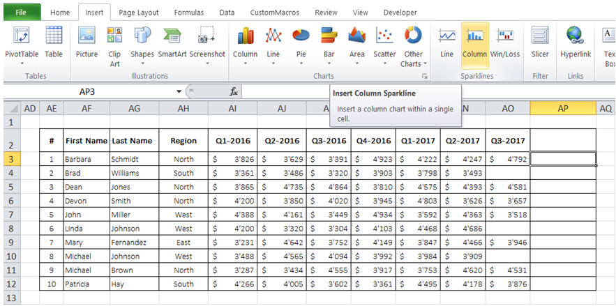
a) Select the cell to the right of last column for first employee. Under "Insert" tab, click on "Column" in "Sparklines" section.

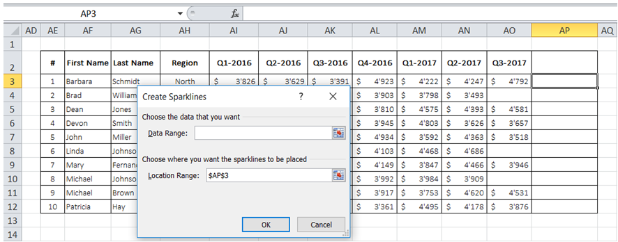
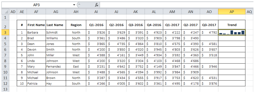
b) "Create Sparklines" dialog box pops up. Enter / Select the range of data for first employee (AI3:AO3) and then click OK.

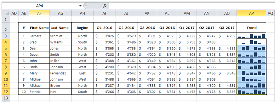
c) A small trend chart is introduced in cell AP3 that is far easier to interpret than reading through data in cells from AI3 to AO3.

d) Copy cell AP3 and paste from AP4 to AP12 to add the charts for the remainaing employees. Charts are added as shown below for every employee.

You can find similar Excel Questions and Answer hereunder

1) How can I add a 3 Month Moving average Trend line to my line chart?

2) How can I add a Footer to my printout with automatic page numbering?

3) How can I enter a picture in a cell?

4) How can I set the fill color, font color and set number format of cell to date?

5) How to find the cell address from the column number in VBA

6) how do you enter multiple line in a cell in Excel

7) Vlookup to return multiple values in same cell in Excel

8) How can I identify the cells that influence a particular cell to help with debugging of my spreadSheet or understand a spreadSheet that I inherited?

9) How can I enter a cent symbol in a cell?

10) How can I find the last used cell in a Column in VBA?