Pivot Tables in Excel
Pivot tables are one of the most useful tool of Excel when you need to go
through big table of data or numbers. This is ideal in this big Data age.
Pivot tables in Excel are quite easy to use once you understand the basic principle. It allow to regroup data that is similar, add rows with the same headers, find sum of columns easily, make relationships between one type of data and another type of data. With a Pivot Table in Excel you can "see" things that are usually hidden in this big amount of data.
Lets take the data from from a Farm Orchard collected over
from 2010 to 2014.
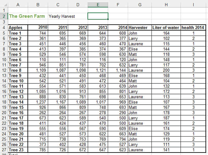
Our excel data includes the amount of apples per tree and per year,
the name of the harvester and the health and number of liter of water the
tree received. With a Pivot table you will be able to see for example which harvester collected the most applesor which apple was the most productive over the years.
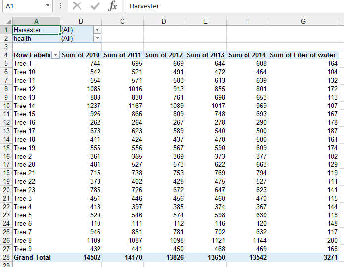
Here the table.
We want to know which Harvest had the most apple over the
years.
So to this we need to make a pivot table that will
agglomerate the various data in this table.
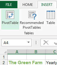
First we select the area we want the table to used the data
from and then we press the PIVOT TABLE button in the INSERT RIBBON.
The Create Pivot Table window will open.
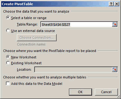
Just make sure the range is correct and press OK.
Usually it is best to create a pivot table in a separate
sheet. Its cleaner.
Automatically, a new sheet is created looking like this.
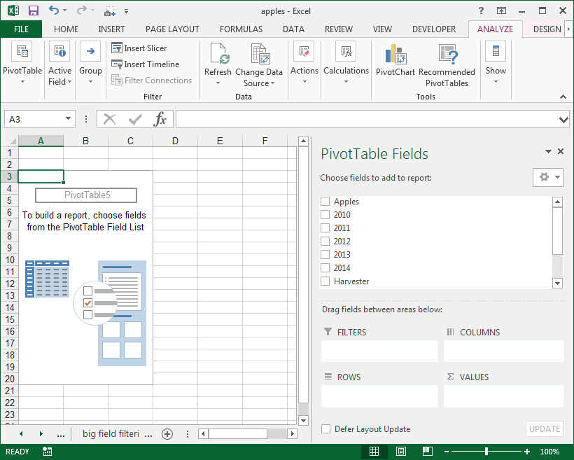
On the right you see the various headers of your table. Now
what we want to do is to MIX correctly these fields and make a new table out
of it.
TIP: YOU NEED TO ASK YOURSELF THE CORRECT QUESTION.
WHAT DO YOU WANT TO DISPLAY.
In our case we said, we want to know what each harvester did
every year.
This means we need to have the harvester names as the
FILTER.
The Trees or Apples will be the ROWS and
the values of each year will be the VALUES.
By Sliding every field into the correct area you get:
and the following table is created.
Now you can see in the A row that Harvester is a field you
can select. Do this:
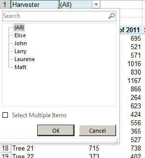
By selecting JOHN, you will see which tree John harvested
over the years and how many apples.
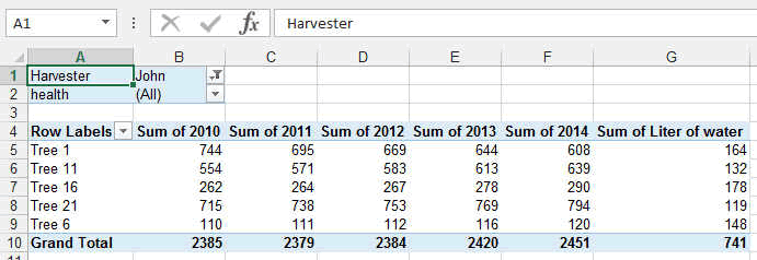
Now you can do this for all the harvesters but you could
have this in one table only.
By changing the filter like this. The harvester is the rows
and the apples are the filter. Or you could just not put the apples.
Following table will appear.
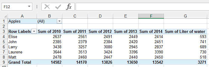
Here you could also compare the number of liters of water
and the health of the tree and see if there is a correlation.
So you can see how easy it is to find some complex data in a
big table using the Excel Pivot Tables.
So that's it for the pivot table
in Excel.
These were only some basics. Now you will learn by doing or
if you want to become a Pivot Table Expert and go into the details and
secrets of pivot tables, you should visit to the site
SpreadSheetTo that has 12 chapters,
has an exercise file, a video - and it's updated for Excel 2016