Conditional Formatting in Excel
Conditional Formatting is, as its name says, the possibility
to format (meaning changing the style, color, etc... of text, cells)
automatically a cell depending of what this value in this cell is.
Let's say, you are rolling a dice and writing the numbers in
Excel.
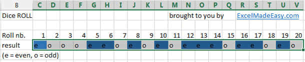
For Even numbers you want the cell to be Blue and for Odd
numbers you want it to be Orange.
If you roll the dice 1000 times, then changing the color
each time manually would be very tedious. That is where Conditional
Formatting intervenes.
Here this example with the table containing the rolls (only
20 for the example). The table is horizontal here just for reading purposes.
Putting the results vertically could be better if you are interesting in
filtering the data on a later stage.
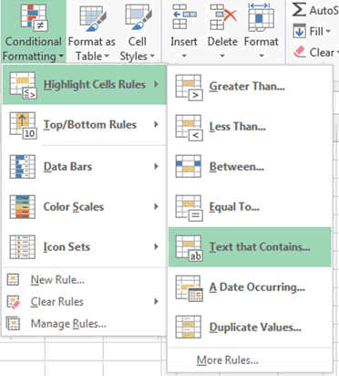
Now we want to select the CONDITIONAL FORMATING
button in the HOME ribbon and we select the Highlight cells rules where the
TEXT contains...
Select all the results.
The following window opens:
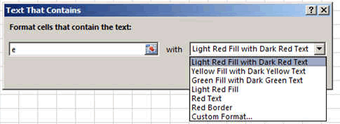
Select CUSTOM FORMAT...
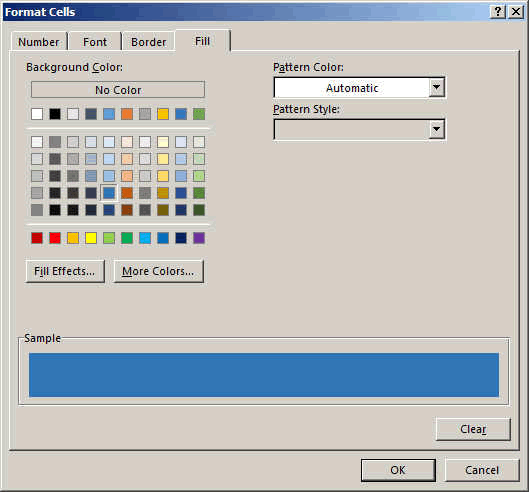
Press OK then OK again.... and this first change will
appear.
Repeat the operation and enter the letter o
instead of e, change the colour to orange and you will get.
This was a very basic Conditional formating.
Vertically this would look like following and you can see
that I changed it into a table so that I can now filter it if I want.
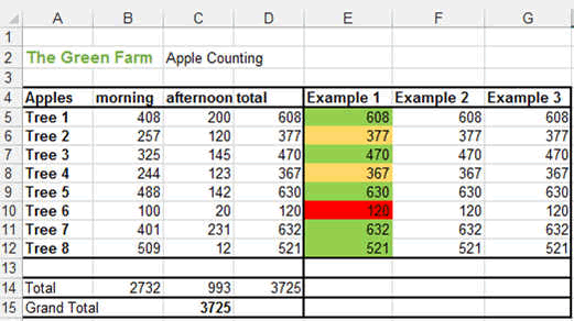
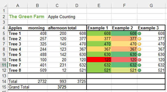
Apple farm
You can see that for our tree counting, we used another Conditional
Formatting which is the Data Bars. In the column E, the blue bars represent
the number of apples.
Isn't this a great way to visualize numbers!!
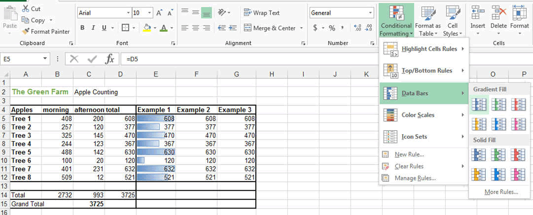
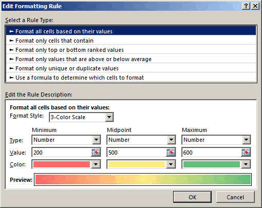
If you wanted to created THREE (3) colors for the apple
quantity, Green over 600 apples, Orange between 200 and 599 and Red under
200, then you would have to create a new rule. In that case the FORMAT ONLY
CELLS THAT CONTAINS part.
Before that you have to SELECT the Cells you want to format.
E5 to E12.
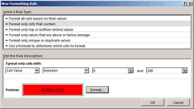
Then enter the minimum value and maximum value.
Select the FORMAT... you want the cells to take.
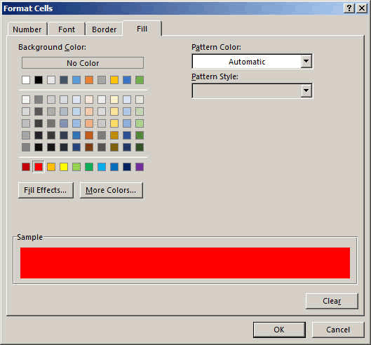
And press OK.
REPEAT this 3 times....
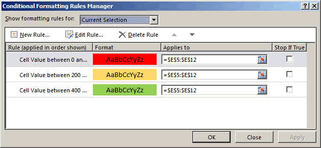
To finally get:
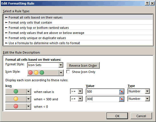
You can change apply other rules and get slightly different
results:
Or this one
To finally get
So that's it for the conditional formatting.
These were only some basics. Now you will learn by doing.