LOOKUP, VLOOKUP, HLOOKUP functions in Excel
What is Vlookup? The Excel lookup functions are used to create formulas to find the specific information you
search in a table. An Excel Array Lookup allows you to lookup values in a table or array.
Vlookup means vertical lookup
Hlookup means horizontal lookup.
Lookup will look in the full table.
In our example we have a sales team and their ID listed from 10 to 15.
The sales are recording the ID only and so our table will add the name of
the sales person beside the sales and ID.
HLOOKUP
Here the first example. Hlookup in Excel looks for a value HORIZONTALLY in an Array.
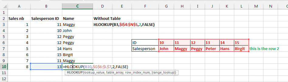
HLOOKUP(the lookup value you are looking for here B10, $G$6:$L$7, 2, FALSE)
=HLOOKUP(The lookup Value you want to look up, range where the value should be, hlookup row index, Exact Match 0/FALSE or Approximate Match 1/TRUE).
Be careful to enter the table array in absolute position (with $x$y).
The number 2 represents the second (2nd) row. This is where the output value
should come once the ID is found.
FALSE means the value should fit the lookup value.
TRUE would mean the result/output value, if not found exactly, could be the
nearest match.
VLOOKUP
Here the second example. VLookup looks for a value VERTICALLY.
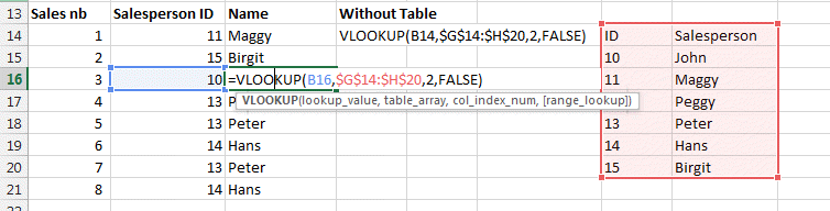
Here the same as before just vertically.
VLOOKUP(value you are looking for here B16,$G$14:$H$20,2,FALSE)
=VLOOKUP(Value you want to look up, range where the value should be, vlookup column index, Exact Match 0/FALSE or Approximate Match 1/TRUE).
The number 2 represents the second (2nd) column, it is the vlookup column index. This is where the output value
should come once the ID is found.
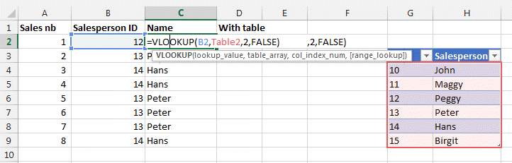
You can also use table if your name and IDs are in a table. Here example
with table2 being this table. THis makes things more easy or readable.
FALSE means the value should fit the lookup value.
TRUE would mean the result/output value, if not found exactly, could be the
nearest match.
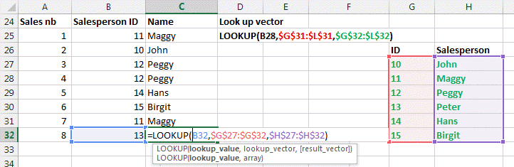
LOOKUP
Lookup looks in the full table or in a selected area of the table (called a
vector).
IMPORTANT: for the LOOKUP function to work correctly, the
data that you are looking into must be sorted in ascending order.
If this is not possible, use VLOOKUP, HLOOKUP or MATCH.
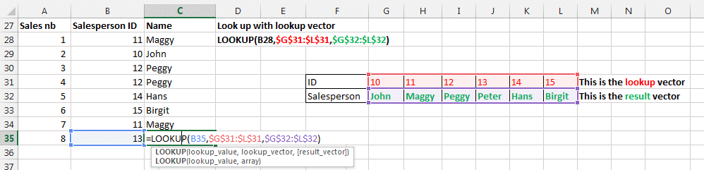
LOOKUP(what you are looking for, lookup vector, result vector)
You can see here the Lookup function looks in the ID row and returns the
Name Row as a result vector.
Same vertically.
Look at the INDEX
(click on the link for details) to
select an item in a list by its coordinates row and column
=INDEX(Range, row, column)
Also the CHOOSE
(click on the link for details) function
allows you to choose 1 item in a list
=CHOOSE(rank of the name to choose (1 or 2 or 3, ...) , name1, name2, name3, name4, .......)
Download the example from here.
TIP: Use the wildcard * and ? in
your formulas. Look in our
tips and tricks
section.
Please Tweet, Like or Share us if you enjoyed.