Top 10 fonctions in Excel. The ones you MUST know.
Here are sumarized the 10 most important functions and formulas that you need to have a good start with Excel.
1) SUM, SUMPRODUCT
2) SUMIF, SUMIFS
3) VLOOKUP, LOOKUP
4) IF
5) Arithmetic formulas, functions and other special characters
6) Networkdays, workday, today()
7) Max, Min, Large, Small, Rank
8) Text Formulas
9) IFERROR
10) Combine MATCH, INDEX: ultimate power in Search
Rank 1: SUM, SUMPRODUCT
Instead of adding cells one by one, the sum function allows you to sum directly a full column or row or area.
= SUM(10,10,20,A2) 10+10+20+A2 = 40+A2
= SUM(A1:A100) the full column from 1 to 100
=SUM(A1:D1) the first row A1+B1+C1+D1
=SUM(A1:D100) all the 400 cells are added from A1 to D100.
The Sumproduct allows you to quickly multiply all the items in a row and then sum up the rows one by one.
Here the quantity x price x margin for every article is added and gives you to the total profit.
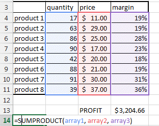
You can find more in the sum product page.
Rank 2: SUMIF, SUMIFS
This is such a useful formula.
It answers the question: how much of product A have we sold in region B and by sales person C in year D (how many TV were sold in America by John in 2012? )
Answer to your boss in a second thanks to Sumifs.
The difference between Sumif and Sumifs is that Sumif only accepts one condition.
=SUMIF(Array you want to sum, array with criteria 1, criteria 1, array with criteria 2, criteria 2, array with criteria 2, criteria 2, ....)
=SUMIFS(D19:D25, B19:B25, "TV", C19:C25, "John")
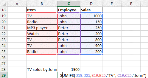
You can find more in the sumif page.
Rank 3: VLOOKUP, LOOKUP
What is common between all VLOOKUP first time users? They are bold because they lost it...
The Lookup function are here to find items in a table.
It is used widely by every Excel User in the world. But it has its limitations you have to know.
VLOOKUP looks for data only in the first column of your table
LOOKUP only uses sorted tables.
The workaround is to use INDEX and MATCH (see rank 10 or this page)
Here how it works.
=VLOOKUP(the value you are lookingfor in the first column, the array it is in, which column you want the result to come from ,FALSE)
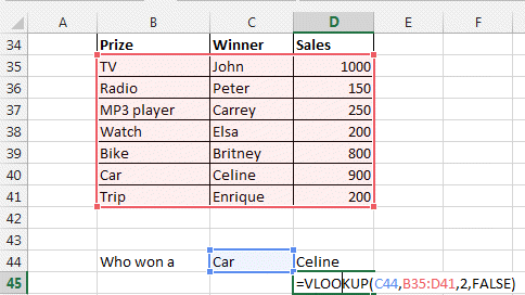

As said, the problem with VLOOKUP is that you can only search the first column and give a result out of any following column.
To get over this hurdle, you should use the LOOKUP function that came with Excel 2003. But it has also limitation. Find how in our Lookup page.
=LOOKUP(Value you are looking for, vector where to look for this data, vector of the data you want to display).
Definition: a vector is a one dimension array or range. For example A1:A4 to B4:G4. You cannot enter a 2 dimension range like A1:G4.
Another way is to use the MATCH and INDEX functions together. See this done in rank 10 or in our INDEX and MATCH page.
Rank 4: IF
The IF function lets you test IF something is true then make something and if it is false then do something else.
=IF(test , value_if_TRUE , value_if_FALSE)
=IF(test , value_if_TRUE or do something else , value_if_FALSE or do something else)
Look at this exemple
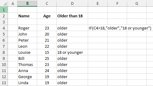
=IF(persons_age > 18, "older", "youger")
You can of course do nesting. This means you can insert another if function into an if.
IF(Persons_name="Leon", if(person_age>18, "Leon is older than 18", "Leon is younger than 18"), "this is not Leon")
and you can go on and on with nesting.
The main operators in the formulas are > bigger, < smaller, = equal, >= bigger or equal , <= smaller or equal, <> different.
Find more details here.
Rank 5: Arithmetic formulas, functions and other special characters
Of course you have to know the basic arithmetic formulas.
+, -, /, *: the basic operators. 2+3+12/4-6*4
%: percentage divides by 100. If you type 4% it will display 4% but the value will be 0.04.
&: To concatenate text. ="John" & " " & "Kennedy" will give John Kennedy
( ): Parenthesis. To separate element. =A1+B2*(C2+4%)
^: Power. To put a number to a power. Like 2^3 = 8. Or 2^(A1+B2).
" ": These are used to write text. "this is text". Used in formulas like IF(A1="Apple", "Steve Job", "Bill Gate")
: : column serves to indicate ranges A1:B3 will include all cells A1, A2, A3, B1, B2, B3. So SUM(A1:B3) will sum this 6 cells.
$: Lock reference of cell. Like =$A$1. Where-ever you copy the cell containing $A$1 it will never change. If you slide it down, it will stay linked to this cell. But =$A1 will lock only the A column, the 1 will change to $A2, $A3, ... if you slide it down. Press F4 to change from one to the other.
{} : defines an array. {1,2,3,4} defines an array of numbers.
[ ] : this refers to the name of one column of a table. Like Table1[sales], this refers to the sales column of the table 1.
* ?: this can be used as wildcard in LOOKUP functions, COUNTIF functions. Look in our tip and tricks section.
<, >, >=, <=: logical operators can also be used in formulas. Example =(6>3)+2 will give result 3. Because =6>3 results in TRUE or 1. So 1+2 = 3. Instead of numbers you can use Cells =(A6>A3)+2 will give 2 or 3 as result depending if A6 is bigger or smaller than A3.